Gradebook analysis with R – Part I

This is Part I in Scout from University of California’s three-part series, Gradebook Analysis with R. You can read Part II here, and Part III here.

Gradebooks are rich sources of information. Hidden among the test, quiz and homework scores often lie important insights into the curriculum and student performance. While assessing a curriculum’s overall effectiveness and integrity is an enormous task that requires much more data, a gradebook’s ability to flag potential issues makes it a useful entry point.

The analytics tools and interfaces provided by learning management systems (LMS), however, are sometimes inadequate. This is not meant as criticism. Data analysis is an imaginative exercise whose questions no LMS provider can fully anticipate. Furthermore, the best questions often require data from additional sources, such as your student information system (SIS). As we hope to demonstrate in this series, joining datasets from a variety of sources, issuing complex queries, and producing compelling data visualizations are tasks for which the R programming language and the environment are well-suited. R is a popular tool among statisticians and data scientists, but recent improvements have made it more accessible to the general public. This tutorial does not cover installing R, but an easy guide can be found here. R also has a fantastic integrative development environment (IDE) called RStudio, but it’s not required for any of the data analysis performed here.

Loading and Viewing Your Gradebook

First, we need our data. Every LMS allows you to export your gradebooks to a comma-separated values (CSV) file, so once you’ve downloaded the desired gradebook CSV onto your computer, you’re ready to open R. A screen shot of our raw data is below:

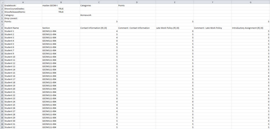
Open R, and at the command line use the setwd() function to move your working directory wherever the gradebook is located. For example, we exported our Geometry gradebook to a directory called “Gradebooks” on our Desktop, so we enter:

setwd(“Desktop/Gradebooks”)#The path to the directory must be in quotation marks.

We can confirm the file is in the directory with the list.files() function. To read the file into R, we’ll use the read_csv() function from the readr package, which, like all R packages, must be installed prior to use with install_packages(“package_name”). In the example below, we’re creating an R object and naming it geometry. The <- operator tells R to assign to geometry whatever is returned by the function on right, which in this case is a table from the CSV file.

install.packages(“readr”)
library (readr) #We need to load the readr package where read_csv() resides
geometry <- read_csv(“geometry_gradebook.csv”, skip = 7)

Note that in the image above, the data we need begins on the eighth row. Thus, the second argument (skip = 7) tells R to skip seven lines before reading the data. Part of the hidden beauty of read_csv() is its speed and default settings. We could have read the gradebook into R with the read.csv() function from base R, but we would then have had to supply additional arguments, such as header = TRUE and stringsAsFactors = FALSE. Without going into detail, the dataset object created by read_csv is superior to what is created by read.csv().

geometry is now an R object, and we can begin to examine it. Towards that end, R has several useful functions:

• dim() prints the dimensions of an R object (e.g., number of rows and columns).
• str() prints the structure of an R object, as well as the column names and the type of each column (e.g., character, numeric, integer, etc.).
• names() prints the names of an R object.
• head() prints the first few parts of an R object.
• tail() prints the last few parts of an R object.

Here are some examples of these functions called on our geometry dataset:

dim(geometry); kable(head(geometry[,11:16])) #kable() is an optional function to format the display

[1] 32 96

[table id=7 /]

Subsetting and Cleaning Your Gradebook

This dataset has 32 rows and 96 columns (i.e., 32 students and 96 variables). For our purposes, we want to focus on the gradebook scores, so we can drop the general information about the students and the columns containing teacher comments. To do so, we’ll use the select() and contains() functions from the handy dplyr package to specify which columns we want to keep. The contains (“Homework”) clause, for example, indicates that we want all columns whose header contains “Homework.”

library(dplyr)
geometry <- select(geometry, #The first argument of select() is the dataset `Student Name`, #Column names with spaces must be closed by backticks
`Calculated Grade`,
contains(“Final”),
contains(“Homework”),
contains(“Quiz”),
contains(“Project”),
contains(“Exam”
-contains(“Comment”)) #”-” tells R to drop columns with “Comment”

Checking the dimensions and column names of our new, smaller dataset, we see that the number of columns has dropped to 42:

dim(geometry); head(names(geometry), 20)

[1] 32 42

[1] “Student Name” “Calculated Grade”
[3] “Final Exam, Form A (R) (0)” “Lesson 1 Homework (R) (0)”
[5] “Lesson 2 Homework (R) (0)” “Lesson 3 Homework (R) (0)”
[7] “Lesson 4 Homework (R) (0)” “Lesson 5 Homework (R) (0)”
[9] “Lesson 6 Homework (R) (0)” “Lesson 8 Homework (R) (0)”
[11] “Lesson 9 Homework (R) (0)” “Lesson 10 Homework (R) (0)”
[13] “Lesson 11 Homework (R) (0)” “Lesson 12 Homework (R) (0)”
[15] “Lesson 13 Homework (R) (0)” “Lesson 14 Homework (R) (0)”
[17] “Lesson 15 Homework (R) (0)” “Lesson 16 Homework (R) (0)”
[19] “Lesson 01 Quiz (R) (0)” “Lesson 02 Quiz (R) (0)”

If you’re picky about column names like us, the extraneous “(R) (o)” at the end of each column name is annoying and should be removed. Furthermore, when we start creating plots across facets and grids in Part II, we’ll want cleaner plot titles. Here we’ll use the str_sub() and str_trim() functions from the stringr package to remove the final eight characters from each column name and trim the remaining white space:

library(stringr)
names(geometry)[3:42] <- str_sub(names(geometry)[3:42], start = 1, end = -8)
#”(R) (0)” only occurs in columns 3-42
#The third argument (end = -8) tells R to remove the final eight characters
names(geometry) <- str_trim(names(geometry))
head(names(geometry), 20)

[1] “Student Name” “Calculated Grade” “Final Exam, Form A”
[4] “Lesson 1 Homework” “Lesson 2 Homework” “Lesson 3 Homework”
[7] “Lesson 4 Homework” “Lesson 5 Homework” “Lesson 6 Homework”
[10] “Lesson 8 Homework” “Lesson 9 Homework” “Lesson 10 Homework”
[13] “Lesson 11 Homework” “Lesson 12 Homework” “Lesson 13 Homework”
[16] “Lesson 14 Homework” “Lesson 15 Homework” “Lesson 16 Homework”
[19] “Lesson 01 Quiz” “Lesson 02 Quiz”

Much better! Our column names are clearer and free of extraneous white space. Here we should note that it’s generally preferable to remove spaces from your column names, and we could do so by calling make.names(names(geometry)). We intend, however, to reshape our data into new columns below, so we can leave the spaces for the time being.

Tidying Your Gradebook

Our column names are clean, but the dataset is not tidy. Tidy data has two key characteristics:

• Each column is a variable.
• Each row is an observation.

While meeting the second condition, geometry violates the first. We have 42 columns, but really only six variables: Student Name, Final Exam Grade, Calculated Grade, Item and Score. You could argue that the Calculated Grade and Final Exam Grade scores could be rolled into the Score variable and that there are only three variables (Student Name, Item, Score), but for our purposes, we want to treat the Calculated Grade and Final Exam Scores as separate variables.

Tidying data is easy with the tidyr package. gather() takes multiple columns and collapses them into what are called key-value pairs. In the example below, we’re taking the 39 assignment columns from geometry (columns 4-42) and collapsing them into two new columns, Item (the key) and Score (the value). The column names will fall into rows under Item, and the scores will fall into rows under Score.

library(tidyr)
tidy_geometry <- gather(geometry, Item, Score, 4:42)

Checking the dimensions of tidy_geometry, we can see that our dataset is now 1248 rows tall and only five columns wide:

dim(tidy_geometry); kable(head(tidy_geometry))

[1] 1248 5

[table id=8 /]

We’re almost ready to begin querying our data. Creating some additional variables will help us issue more incisive queries and can be accomplished with a combination of the mutate(), ifelse() and grepl() functions. mutate() adds a new variable to a dataset, ifelse() tests a logical condition and returns TRUE or FALSE, and grepl() searches for matches within a character vector. In the example below, we’re creating two new variables, Type and Result. If “Homework” appears within the Item name of a particular row, its Type becomes “Homework.” If “Quiz” appears within the Item name of a particular row, its Type becomes “Quiz,” and so on and so forth. Result is the second variable created, and is dependent on the student’s Calculated Grade:

tidy_geometry <- mutate(tidy_geometry,
Type =
ifelse(grepl(“Homework”, Item), “Homework”,
ifelse(grepl(“Quiz”, Item), “Quiz”,
ifelse(grepl(“Project”, Item), “Project”,
ifelse(grepl(“Exam”, Item), “Exam”, “Other”)))),
Result =
ifelse(`Calculated Grade` > 60, “Passed”, “Failed”))

Stepping back and reviewing our code, we could have rewritten the script in a more succinct fashion with the %>% operator from the magrittr package. %>% “pipes” the R object to its left into the function on its right, allowing you to chain multiple functions together. The technique not only reduces the amount of code you need to write but also improves its readability. It may help to think of %>% as a synonym for “then,” as in, first take geometry, then do this, then do this, etc.

The %<>% operator is a handy combination of <- and %>%: it both assigns and pipes.

library(readr)
library(stringr)
library(dplyr)
library(tidyr)
library(magrittr)

geometry <- read_csv(“geom111004.csv”, skip = 7) %>%
select(`Student Name`, `Calculated Grade`, contains(“Final”), contains(“Homework”),
contains(“Quiz”), contains(“Project”), contains(“Exam”),
-contains(“Comment”))

names(geometry)[3:42] %<>%
str_sub(1, -8) %>%
str_trim()

tidy_geometry <- geometry %>%
gather(Item, Score, 4:ncol(.)) %>%
mutate(Type =
ifelse(grepl(“Homework”, Item), “Homework”,
ifelse(grepl(“Quiz”, Item), “Quiz”,
ifelse(grepl(“Project”, Item), “Project”,
ifelse(grepl(“Exam”, Item), “Exam”, “Other”)))),
Result =
ifelse(`Calculated Grade` > 60, “Passed”, “Failed”)) %>%
rename(Final = `Final Exam, Form A`, #Retaining spaces in column names is unadvisable
Grade = `Calculated Grade`,
Student = `Student Name`)

Joining Other Datasets to Your Gradebook

We could start analyzing our gradebook now, but joining data from our SIS will enrich the dataset and further sharpen our analysis. At Scout we obtain information about a student’s gender, their parents’ education levels, whether they have an IEP or 504 plan, and whether they attend a public or private school, among other variables. This mix of categorical and quantitative variables makes for a rich and interesting dataset.

In the example below, we’ve downloaded another CSV file from our SIS onto our desktop. Using the setwd() and read_csv() functions again, we’ll move our working directory back to the desktop, read the file into R, and join the new dataset, sis_data, with geometry:

setwd(“..”) #Shorthand meaning “move back one directory”
sis_data <- read_csv(“sis_data.csv”)
rich_geometry <- left_join(tidy_geometry, sis_data, by = “Student”) #sis_data must also have a matching Student column

There are many different ways to join tables. By calling left_join(), we’re matching all the rows from geometry with corresponding rows from sis_data. The third argument (by = “Student”), indicates which column to join by. For more about joins and relational data in R, Garrett Grolemond and Hadley Wickham created a terrific overview here.

Querying and Summarizing Your Gradebook

To recap: we’ve (1) loaded, subsetted and cleaned our gradebook, (2) reshaped our gradebook from long to tall, (3) created two additional variables, (4) renamed some variables to remove the spaces, and (5) added variables from our SIS. A brief summary of our variables in the cheesily named rich_geometry can be obtained with str():

str(rich_geometry)

Classes ‘tbl_df’, ‘tbl’ and ‘data.frame’: 1248 obs. of 9 variables:
$ Student : chr “Student 1” “Student 2” “Student 3” “Student 4” …
$ Grade : num 1.4 60.8 68.6 60.2 66.5 …
$ Final : int 0 90 69 63 71 122 84 135 101 60 …
$ Item : Factor w/ 39 levels “Lesson 1 Homework”,..: 1 1 1 1 1 1 1 1 1 1 …
$ Score : num 0 16.2 19.4 15 14.9 20 14.8 18.6 20 13.3 …
$ Type : chr “Homework” “Homework” “Homework” “Homework” …
$ Gender : chr “Female” “Male” “Female” “Male” …
$ Parent_Education: chr “Non-College Grad” “Non-College Grad” “Non-College Grad” “Non-College Grad” …
$ Result : chr “Failed” “Passed” “Passed” “Passed” …

We’re now ready to begin querying and summarizing our dataset. Here there is no limit to the questions we can ask, and some additional functions from the dplyr package help us create quick and easy queries:

• filter() returns rows with matching conditions (e.g. Score > 70).
• group_by() groups data into rows with the same values.
• summarize() summarizes multiple values to a single value
• arrange() arranges rows by variable in either ascending or descending order
• distinct() retains only unique rows of a variable

Sample Questions and Answers

Question: which students performed best on quizzes?

rich_geometry %>%
filter(Score > 0, Type == “Quiz”) %>% #We want to filter 0s, which indicate missing assignments
group_by(Student) %>%
summarize(Quiz_Mean = round(mean(Score), 2)) %>% #round() rounds the values to two decimal places
arrange(desc(Quiz_Mean)) %>% #Display Quiz_Mean in descending order
head() %>% #Display only the first six rows
kable() #Format the table display

[table id=9 /]

Answer: Students 27, 8, 30, 11, 6, and 26

Question: What are the summary statistics of each exam?

rich_geometry %>%
filter(Score > 0, Type == “Exam”) %>%
group_by(Item) %>%
summarize(Mean = mean(Score),
Median = median(Score),
Std_Dev = sd(Score)) %>% #sd() computes the standard deviation
kable()

[table id=10 /]

Answer: (See above)

Question: Did either gender outperform the other on quizzes or exams?

rich_geometry %>%
filter(Score > 0, Type == “Exam” | Type == “Quiz”) %>% #”|” indicates all rows with exams OR quizzes
group_by(Gender, Type) %>%
summarize(Mean_Score = round(mean(Score), 2)) %>%
kable()

[table id=11 /]

Answer: Yes, males outperformed females on both quizzes and exams.

Question: Which gradebook items are least correlated to final exam performance?

rich_geometry %>%
group_by(Item) %>%
summarize(Correlation_to_Final = round(cor(Score, Final), 2)) %>% #cor() computes the correlation
arrange(Correlation_to_Final) %>%
head() %>%
kable()

[table id=12 /]

Answer: The projects, as well as the homework from lessons 5, 15, and 12.

Question: Did students whose parents graduated from college pass the course at a higher rate?

rich_geometry %>%
distinct(Student) %>%
group_by(Parent_Education) %>%
summarize(Pass_Percentage = round(mean(Result == “Passed”), 2)) %>%
kable()

[table id=13 /]

Answer: Yes, students whose parents graduated from college passed the course at a higher rate.

Again, it would be impossible for any LMS to anticipate all of these questions in advance. With just a few lines of code, we can explore our data with imaginative freedom. In Part II, we’ll continue our exploratory data analysis by building scatter plots, box plots and histograms. R has fantastic graphing capabilities that help us create compelling visualizations and dashboards.

Have a question about R or this tutorial? Feel free to email me at [email protected].

About the Author

David wrangles, slices and dices data for Scout, but he also likes to pal around with the English department reciting Julius Caesar, extolling the innumerable merits of East of Eden and arguing about the hegemonic canon.

About Scout

Learning is synonymous with empowerment at Scout. We are teachers, instructional designers and technologists working to deliver University of California-quality interactive online classes, curriculum and supplemental education materials to middle school and high school students and teachers across the U.S. and beyond. Our course materials are designed to inspire lifelong curiosity and prepare pupils of all backgrounds and education levels for an increasingly technological world where training and job skills are mobile, asynchronous and self-directed. Explicitly created to bridge achievement gaps, we believe that using technology effectively can remove traditional obstacles to education.