Executive Summary
In this project we explored student behavioral, textual, and limited demographic data retrieved from Michigan Virtual School for the 2014-2015 and 2015-2016 academic years. One overarching goal was to determine the type of data we could collect as well as how accurate and comprehensive that data were. We also wanted to explore a variety of data mining analysis techniques, including deep learning (DL) for text analysis and improved prediction accuracy. Specifically, we were interested in comparing DL to other machine learning (ML) models, as well as exploring the potential of DL combined with textual data in improving prediction accuracy. Finally, we were interested in looking for predictors that could act as early warning indicators for detecting learners that might be at risk of failure early in the semester.Our results indicate that DL was slightly better than other ML models, and the inclusion of textual content improved the overall predictive accuracy in identifying at-risk students. Although the percentage was a relatively small increase in prediction power when using DL, this increase adds an additional element of accuracy in our efforts to use data to support learners, and in particular, at-risk learners. Perhaps the most important finding was our ability to achieve accurate prediction power with a relatively high level of generalizability and stability. The question of generalizability is important because it may allow us to use the model across different contexts.In addition to an increase in predictive power, we used a surrogate model analysis to assist us in identifying a predictive variable. One of the Singular-Value Decomposition (SVD 6) features from the text analysis was identified as an important feature for identifying at-risk students. We tried a variety of approaches in examining the raw text from this feature and discovered some commonalities. Successful students were all enrolled in the Government class while at-risk students were enrolled mostly in the Civics class. Further analysis of the SVD 6 threshold predictor revealed that first semester courses, courses with 20 or fewer enrollments, and courses in the disciplines of History, Geography, and Political Science all demonstrated larger percentages of predicted at-risk students. We also analyzed the raw text data itself to see if we could tease out a meaningful explanation for the importance of this predictor. Although a variety of meanings might be attributed to the underlying cause of this textual feature being identified as a significant predictor in the DL analysis, at this point everything is conjecture.
Recommendations
Based on our initial data mining explorations with DL, we make the following recommendations:
Continue exploring the DL model which resulted in an overall prediction accuracy of 86.9%, a prediction accuracy of 94.5% in identifying successful students, and a 54.5% in identifying at-risk students. The results show a slight increase in the accuracy of predicting at-risk students. However, even just 1% additional predictive power is worth the extra effort of DL.
Increase the number of courses used in the data set. The access to course data in the current study was intentionally limited. The model may change with additional course disciplines. It is also the case that if all course data were used, the accuracy might be improved. Smaller data sets prohibit “deeper” levels of analysis using more advanced DL methods.
Seek to advance generalizability of the model. For example, even though it is more challenging, generating relative frequency across courses improves generalizability. However, deriving relative frequency across the limited courses to which we had access required extensive code, so deploying across an entire institution would be very complex. There are other ways we can test for generalizability. We could compare results with data from another set of course categories or domains identified as important to the institution or compare with the entire set of course offerings.
We know SVD 6 is an important association with performance, but we don’t yet know why. Continued research into data mining with the inclusion of text mining would be an important next step. For this study we applied Natural Language Processing (NLP) to the SVD approach to extract the textual features. There are other more advanced methods we can try such as variant auto-coder or t-distributed stochastic neighbor embedding (t-SNE). New research may also offer further prediction power including the work by Pennebaker, Chung, Frazee, Lavergne, and Beaver (2014) in using function words as a predictor of success.
Differentiate discussion post text by teacher/student within a single thread if possible to improve the quality of the data (removing noise).
Investigate DL with text mining in real-time Time Series Analysis validation.
When setting parameters for identifying at-risk learners, the limitations of the model suggest that it is better to err on the side of over identifying.
To improve the prediction accuracy and generalizability of the model, identify more variables highly related to the target status. In other words, link data such as demographics which are more typically indicative of at-risk status such as free and reduced lunch or a school or district level at-risk designation. However, it may be worthwhile to compare models that incorporate this additional data and those that don’t to identify any bias in the algorithm. Labeling or tracking students by profiling can result in the denial of opportunities to underrepresented groups.
The quality of some data was of limited use because of input errors. Providing a drop down with possible choices for student age, rather than allowing students or others to input data by hand is one way to alleviate this problem. Other examples include linking data from one system to another such as additional demographic data with behavioral data in the LMS and linking to other student performance data systems or course evaluation data.
Extracted early warning indicators, including behaviors and number of words posted, suggest that students who accessed materials outside the LMS (ranked lower than 17.03%) and posted fewer words in the discussion forums (ranked lower than 27.53%) had a higher chance of identifying as at-risk.
To improve predictive power in the model, we would suggest collecting more student demographic data at the stage of new student registration.
Project Overview and Goals
For this project we were interested in incorporating emerging deep learning (DL) techniques to develop multiple supervised and unsupervised predictive models in an educational setting. DL is a subset of machine learning (ML), inspired by artificial neural network structures that rely on hierarchical learning of features which become more complex at higher levels. In general, more traditional predictive models need to be highly customized to achieve accurate results. They are dependent on the unique contextual factors in educational settings. For example, frequencies, such as frequency of logins and frequency of course access, are often represented in absolute numbers and highly dependent on how the course is taught. If a predictive model is constructed based on the absolute numbers, the model might become useless when the course is changed, redesigned, or taught by a different instructor. In addition, the absolute numbers are hard to generalize (i.e. transferred to other courses or other institutions). Gašević, Dawson, Rogers and Gašević (2016) argue that there are no models that can accurately predict student performance without taking into account the context of the individual course, specifically, how the technology is used as well as the disciplinary differences. Their findings revealed that out of nine different courses from four disparate disciplines studied, they found no identical predictors of student success. However, DL techniques may offer new possibilities to make generalization possible across different contexts. We postulate that because DL consists of many neurons, those individual neurons might be sensitive to specific features that are ignored by other ML algorithms. This is, in essence, a paradigm shift in our understanding of the potential for ML. We now have the capacity for adaptive analytic models that can “learn” on their own with exceptional predictive power.Following the more common methods of educational data mining (EDM), we included both online learning behaviors and student demographics with DL techniques in this study. However, we extended our investigations to include online discussion content (text) as input variables. Du, Yang, Shelton, Hung and Zhang (2018) reviewed 1,049 Learning Analytics articles published from 2011 to 2017 and identified 317 actual analysis articles (many articles were focused on discussing frameworks or proofing concepts) for further analysis. Prediction of performance generated the greatest number of articles with 52 published articles and 35 conference proceedings from 2011 to 2017. In these 87 articles, the most common input variables included online learning behaviors, student’s educational records, demographics, textual data of online discussions, facial expression, and self-report data. Ninety-two percent of these articles included online behavioral data as input variables. Forty-six percent included online learning behaviors only, and the remainder (54%) combined online learning behaviors with student’s demographics, student’s educational records, and self-report data. Only seven articles (8%) utilized non-behavioral data as input variables. Of the seven, three adopted textual data of online discussions or facial expression, and the remaining four articles combined online textual discussions or facial expressions with student demographics. Although textual data from online discussions is a crucial part of online learning behaviors, there were no studies found that combined online behaviors with textual discussions in the performance prediction model.One of the key elements in successful data mining applications is understanding institutional needs. In educational contexts this encompasses setting strategic administrative and teaching goals and evaluating their impact. However, we approached this initial project in an exploratory stance rather than an approach focused on answering a single question or set of questions. First, we were interested in learning how accessible, comprehensive, and accurate the data were. Second, we wanted to explore a variety of data mining analysis techniques, including DL for text analysis and improved prediction accuracy. And third, we were interested in exploring the potential for predictors that occurred early enough in the semester to act as an early warning indicator for at-risk students.
Data Collection and Analysis Methods
Data Collection and Processing
Data were collected from a subset of online courses offered through Michigan Virtual School (MVS). The major data sources for this project included: (1) student behavioral data: student’s behaviors performed on the Learning Management System (LMS); (2) student demographic data: includes age and gender; (3) textual content: student discussion text posted on the course discussion boards. The Blackboard server logs contained courses in the 2014-2015 and 2015-2016 academic years and resulted in the following raw data and data after cleaning:
2014-2015: 6,941,962 logs (6,701,434 logs after initial cleaning with 5,928 students in 337 course sections)
2015-2016: 8,370,351 logs (8,249,934 logs after initial cleaning with 6,941 students in 343 course sections)
In order to provide a manageable level of data for collection, processing, and analysis in this exploratory study, the number and type of courses were limited and determined by the MVS database administrator. A total of 76 unique courses were selected from 2014-2015 and 67 unique courses from 2015-2016. The following SQL codes show the range of courses that were selected for this project:
course_name like '%History%' or course_name like '%logy%'

or course_name like '%chem%' or course_name like '%sci%'

or course_name like '%econ%' or course_name like '%phys%'

or course_name like '%gov%' or course_name like '%omy%'

or course_name like '%civics%' or course_name like '%space%'

or course_name like '%graphy%' or course_name like '%philoy%'

or course_name like '%culture%'
SAS Enterprise Guide analytics application was used for LMS log data processing of behavioral and textual data. The behavioral data were extracted from the Blackboard activity accumulator which tracks click-by-click actions occurring in the Blackboard LMS. Textual data were extracted from blackboard discussion forums. Figure 1 shows the data processing flows for aggregating and deriving variables. In the first round of data cleaning, all behavioral data were aggregated by behavioral labels defined by Blackboard and stored in the activity accumulator table in Blackboard’s database system (please see Table 1). More detailed information about the database schedule and fields can be retrieved from the following link: http://library.blackboard.com/ref/3ce800bc-d993-40d2-8fc3-1cb792408731/index.htm. A unique ID, combining student ID and course ID, was used to link all three types of data sources together. In order to enhance the model’s generalizability, all behavioral frequencies were converted into “relative values.” Because the requirements of different courses may vary, how often students are required to access course materials or post to discussion forums for example, it is more meaningful to convert student’s participation level from absolute frequency numbers into relative values, such as student’s ranking and ratio by frequencies. Finally, in order to achieve the extended goal of early warning prediction, all input variables were computed from the beginning of the semester to the end of the eighth week in each semester. Table 1 shows the list of variables identified after two rounds of data processing and derived variable generation.
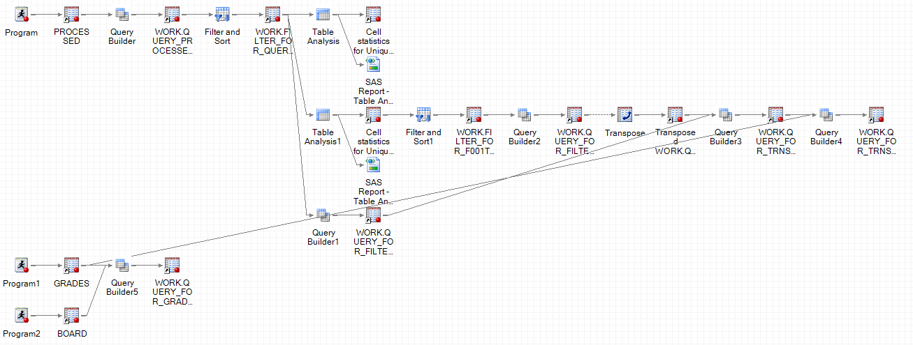
Figure 1. Data processing flow for aggregating and deriving variables.Table 1.
Variables | Description |
|---|---|
Unique_ID | A unique ID to link different kinds of data sources |
course_cate1 | Course coding by offering |
course_cate2 | Course coding by discipline |
course_cate3 | Course coding by enrollments |
Ra_announcements_entry | Student’s frequency ratio in announce entry within the course |
Ra_blank | Student’s frequency ratio in blank within the course |
Ra_content | Student’s frequency ratio in content within the course |
Ra_discussion_board_entry | Student’s frequency ratio in blank within the course |
Ra_check_grade | Student’s frequency ratio in discussion board entry within the course |
Ra_messages | Student’s frequency ratio in check grade within the course |
Ra_db_thread_list_entry | Student’s frequency ratio in thread list entry within the course |
Ra_view_attempts | Student’s frequency ratio in view attempts within the course |
Ra_staff_information | Student’s frequency ratio in staff information within the course |
Ra_db_collection_entry | Student’s frequency ratio in db collection entry within the course |
Ra_notification_settings_caret | Student’s frequency ratio in notification setting within the course |
Ra_my_announcements | Student’s frequency ratio in my announcement within the course |
Ra_display_notification_settings | Student’s frequency ratio in display notification within the course |
Ra_db_thread_list | Student’s frequency ratio in db thread list within the course |
Ra_db_collection | Student’s frequency ratio in db collection within the course |
Ra_discussion_board | Student’s frequency ratio in discussion board within the course |
Ra_hit_count | Student’s frequency ratio in hit count within the course |
Ra_discussion_word_counts | Student’s frequency ratio in discussion word count within the course |
Rr_announcements_entry | Student’s frequency rank in announce entry within the course |
Rr_blank | Student’s frequency rank in blank within the course |
Rr_content | Student’s frequency rank in content within the course |
Rr_discussion_board_entry | Student’s frequency rank in blank within the course |
Rr_check_grade | Student’s frequency rank in discussion board entry within the course |
Rr_messages | Student’s frequency rank in check grade within the course |
Rr_db_thread_list_entry | Student’s frequency rank in thread list entry within the course |
Rr_view_attempts | Student’s frequency rank in view attempts within the course |
Rr_staff_information | Student’s frequency rank in staff information within the course |
Rr_db_collection_entry | Student’s frequency rank in db collection entry within the course |
Rr_notification_settings_caret | Student’s frequency rank in notification setting within the course |
Rr_my_announcements | Student’s frequency rank in my announcement within the course |
Rr_display_notification_settings | Student’s frequency rank in display notification within the course |
Rr_db_thread_list | Student’s frequency rank in db thread list within the course |
Rr_db_collection | Student’s frequency rank in db collection within the course |
Rr_discussion_board | Student’s frequency rank in discussion board within the course |
Rr_hit_count | Student’s frequency rank in hit count within the course |
Rr_discussion_word_counts | Student’s frequency rank in discussion word count within the course |
RN_announcements_entry | Student’s frequency rank ratio in announce entry within the course |
RN_blank | Student’s frequency rank ratio in blank within the course |
RN_content | Student’s frequency rank ratio in content within the course |
RN_discussion_board_entry | Student’s frequency rank ratio in blank within the course |
RN_check_grade | Student’s frequency rank ratio in discussion board entry within the course |
RN_messages | Student’s frequency rank ratio in check grade within the course |
RN_db_thread_list_entry | Student’s frequency rank ratio in thread list entry within the course |
RN_view_attempts | Student’s frequency rank ratio in view attempts within the course |
RN_staff_information | Student’s frequency rank ratio in staff information within the course |
RN_db_collection_entry | Student’s frequency rank ratio in db collection entry within the course |
RN_notification_settings_caret | Student’s frequency rank ratio in notification setting within the course |
RN_my_announcements | Student’s frequency rank ratio in my announcement within the course |
RN_display_notification_settings | Student’s frequency rank ratio in display notification within the course |
RN_db_thread_list | Student’s frequency rank ratio in db thread list within the course |
RN_db_collection | Student’s frequency rank ratio in db collection within the course |
RN_discussion_board | Student’s frequency rank ratio in discussion board within the course |
RN_hit_count | Student’s frequency rank ratio in hit count within the course |
RN_discussion_word_counts | Student’s frequency rank ratio in discussion word count within the course |
Gender | Gender F and M |
Grade | Grade: 1: at-risk; 1: successful |
Variables for Analysis
Simple Data Exploration After Data Cleaning
We made the assumption that traditional statistical analytics were commonly reported so we focused on simple data exploration here.
Demographics
Demographic data was limited to gender. The data for age contained numerous input errors (ranging from -1 to 115), so we removed age from the analysis. Gender was evenly matched across the two academic years in the study, with females being approximately two-thirds of total enrollments (see Table 2).Table 2.
2014-2015 | 2015-2016 | |
|---|---|---|
Female | 62% | 63% |
Male | 38% | 37% |
Gender
Final Grades
Unbalanced data is a challenging issue in ML. Unbalanced data means the target cases (at-risk students) represent only a very small portion in the population compared with the non-target cases (successful students). Therefore, “at-risk” students were defined as those who had obtained lower than a final grade of 65 in the class, an increase over the traditional 60 that is used to signify a passing score. Cases categorized as at-risk using 65 as the cutoff were about 18% in 2014-2015 and 17% in 2015-2016 (see Table 3). This action can significantly increase the model’s performance by alleviating negative effects from the unbalanced data. Records without final grades were removed for later analysis.Table 3.
2014-2015 | 2015-2016 | |
|---|---|---|
>=90 | 36% | 41% |
<90 | 27% | 26% |
<80 | 14% | 13% |
<70 | 5% | 3% |
<65 (at risk) | 18% | 17% |
Final grades
Dimension Reduction
The curse of dimensionality refers to the issues associated with high dimensional data in the data analysis. As the number of dimensions increases, the available samples under each of those dimensions become sparse. This sparsity is problematic for any method that requires statistical significance. For example, if variable A has two values (such as Yes and No), variable B has five values, and variable C has seven possible values, the number of dimensions is 2*5*7= 70. In order to avoid the curse of dimensionality, courses were consolidated by domain areas including discipline, enrollments (class size), and offering type. The domain of discipline was derived by grouping courses from similar disciplines. For example, American History 1A and American History B were grouped into the “history” discipline. An offering is a derived grouping of courses based on how and when a course was offered. Four groups were derived including AP (advanced courses), S1 (first semester offering), S2 (second semester offering) and O (no distinguishable offering). Finally, courses were grouped by the number of enrollments. En1 designates a course with 0-20 enrollments, En2 a course with 21-75 enrollments, En3 a course with 76-200 enrollments, and En4 a course with greater than 200 enrollments. As a general rule, we used major breaks in enrollment patterns to guide our enrollment category indicators. The three derived domains across all courses in our datasets for 2014-2015 and 2015-2016 are highlighted in Appendix A.
Text processing
In order to test whether text posted in discussion forums by students was an important predictor or might have an impact on prediction accuracy, all textual content was converted into vectors. Forty-two features were extracted to represent unique characteristics of student’s textual content in the vector space. These features worked as part of the input variables with behavioral and demographic data in the predictive modeling. These textual features were combined with behavioral and demographics by the unique ID (student ID+courseID).On a completely exploratory investigation, we also conducted an examination of the words within the textual content using the Linguistic Inquiry and Word Count (LIWC) function word analytic tool (Pennebaker, Chung, Frazee, Lavergne, & Beaver, 2014); Tausczik & Pennebaker, 2010). The premise behind LIWC is to focus on how students think rather than on the meaning of what they write. In short, LIWC is a tool used to count the use of function words in student writing samples. Function words have been shown to be reliable indicators of psychological states. For example, pronoun use is reflective of a focus on one’s self, auxiliary verbs suggest a narrative style of language usage, articles are associated with concrete and formal writing, and prepositions are associated with cognitive complexity (Pennebaker, et al, 2014, p.2). In general, text that is heavy in prepositions and articles demonstrates a “categorical” language style indicative of heightened abstract thinking and cognitive complexity. Text containing a greater use of pronouns, auxiliary verbs, adverbs, conjunctions, impersonal pronouns, personal pronouns, and negations is associated with a more “dynamic” language style (p. 6). The use of categorical language styles has been consistently linked with higher academic performance, while dynamic language has not (Pennebaker, et al, 2014; Robinson, Navea, Ickes, 2013).
Regular Machine Learning Models
DL is a subset of ML, inspired by artificial neural network structures that rely on hierarchical learning of features which become more complex at higher levels (Bengio, 2012; Schmidhuber, 2014). The term “deep” means the hidden layer is over three. The first layer, the input layer, is reserved for the input variables. For example, if there are 20 input variables, the input layer will contain 20 neurons (1 neuron = 1 variable). The second layer is the hidden layer. The structure of the hidden layer including the number of neurons, the number of layers, and activation functions is determined by the analyst and used for feature learning. The third layer is the output layer and generates the outcomes. Ensemble models and Neural Network-like models were considered as better models in this classification. Ensemble models use meta-algorithms (i.e. multiple learning algorithms) to obtain better predictive performance than could be obtained from one algorithm alone (Raczko & Zagajewski, 2017; Smolyakov, 2017). Therefore, the following models: Random Forest, Support Vector Machine (SVM) with sigmoid kernel, SVM with Polynomial kernel, SVM with Gaussian Radial Basis Function, and Neural Network were adopted in the analysis.
Data Analysis
Model training
Multiple model competition is a common approach in ML. Because each model has its own strengths and weaknesses in handling data, multiple model competition is an approach to select the best model based on the model’s prediction performance. In order to ensure the model’s prediction capability on unknown data in the future, the best model is the one with the lowest mean of squared errors (numerical target variable) or misclassification rate (categorical target variable) on the validation dataset. For this study, three rounds of data analysis were conducted using the combined 2014-2015 and the 2015-2016 data. In the analysis, 70% of data were randomly selected as the training data (stratified sampling); the remaining 30% were used for model validation. We tried other data splitting percentages and found 70/30 could generate both accurate and stable results. The best model was selected based on the lowest validation misclassification rate. While Enterprise Guide was used for data processing, SAS Enterprise Miner and Python + Tensorflow were used for model training and ML analysis.
Round One
The first round of input data included behavioral and demographic data only. SAS Enterprise Miner 13.1, a well-known ML tool, was used to conduct the analysis. Figure 2 below shows the analytic flows in the SAS Enterprise Miner (Behavioral + Demographics only).
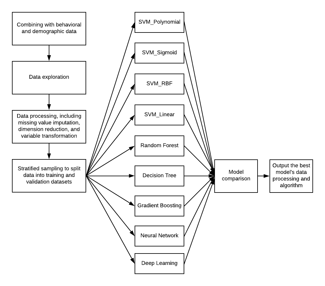
Figure 2. Analytic flow in SAS Enterprise Miner with behavioral and demographic data only.
Round Two
In the second round we aimed to test whether DL could generate better outcomes. The same training and validation datasets were imported into the Python+TensorFlow platform. Figure 3 shows the design of the neural network architecture. The DL network contains two hidden layers. Each hidden layer contains 1,000 neurons. L2 regularization and dropout were enabled to alleviate the issue of over fitting. We also tried to add more layers (going deeper), but these models generated worse results due to the overall fitting caused by the small sample size.
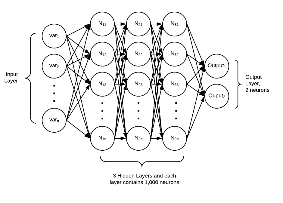
Figure 3. Neural network architecture using Python+TensorFlow with behavioral and demographic data only.
Round Three
The third round included textual features and behavioral and demographic data as input variables. Figure 4 shows the analytics flow for the ML and DL analysis. The DL architecture is still the same as that in the second round.
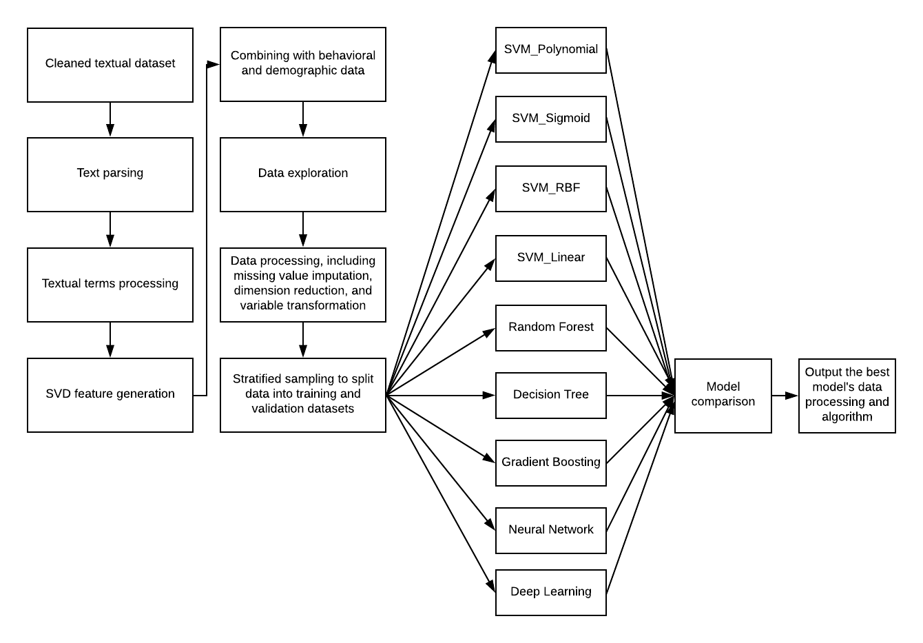
Figure 4. The analytic flow with textual, behavioral, and demographic data.
Model Selection
The confusion matrix is the most popular method to evaluate a model’s performance. The best model is then selected based on parameters (Powers, 2011). After all three rounds of data analysis were completed, we tested for the best model. Using a confusion matrix, four parameters (i.e. True Positive (TP), True Negative (TN), False Positive (FP), and False Negative (FN)) are often used to compute model performance indicators. In this project, “positive” represents at-risk and “negative” represents successful students. TP denotes the number of positive cases captured by the model. TN denotes the number of negative cases captured by the model. FP denotes the number of negative cases misjudged by the model (false early warning). FN denotes the number of positive cases misjudged by the model (missed at-risk students). Two indicators -- accuracy and recall -- were used to evaluate the model’s performance. The formulas are listed below:Accuracy (ACC):TP + TN = _ TP + TN_____ P + N TP + TN + FP + FNSensitivity, recall, hit rate, or true positive rate (TPR):TP = _ TP__ P TP + FNAccuracy represents a model’s prediction performance on both positive and negative cases. Recall is the ratio of positive cases captured by the predictive model. Table 4 shows performance indicators in all three rounds.Table 4.
Tool | TN % | TP % | FN % | FP % | Data | Accuracy | Recall |
|---|---|---|---|---|---|---|---|
Round 3: Deep Learning (Training) | 0.785 | 0.115 | 0.074 | 0.027 | Behavioral + Demographics + Textual Data | 0.899 | 0.607 |
Round 3: Deep Learning (Validation) | 0.766 | 0.103 | 0.086 | 0.045 | Behavioral + Demographics + Textual Data | 0.869* | 0.545* |
Round 3: Multiple model competition (Training) | 0.759 | 0.110 | 0.102 | 0.029 | Behavioral + Demographics + Textual Data | 0.869 | 0.519 |
Round 3: Multiple model competition (Validation) | 0.754 | 0.114 | 0.098 | 0.034 | Behavioral + Demographics + Textual Data | 0.868 | 0.538 |
Round 2: Deep Learning (Training) | 0.767 | 0.110 | 0.102 | 0.020 | Behavioral + Demographics | 0.877 | 0.518 |
Round 2: Deep Learning (Validation) | 0.759 | 0.108 | 0.104 | 0.029 | Behavioral + Demographics | 0.868 | 0.510 |
Round 1: Multiple model competition (Training) | 0.765 | 0.100 | 0.112 | 0.023 | Behavioral + Demographics | 0.866 | 0.473 |
Round 1: Multiple model competition (Validation) | 0.765 | 0.103 | 0.109 | 0.023 | Behavioral + Demographics | 0.868 | 0.488 |
Performance Indicators in Three Rounds of AnalysisNote: *Best model selected.Comparing the first round and the second round, the results indicate that DL performance is slightly better than other ML models (i.e. SVM with Polynomial kernel) in the SAS Enterprise Miner on the recall rates. This means that DL performed better in identifying at-risk students. Overall, DL model’s prediction accuracy is 86.9% with a prediction accuracy of 94.5% in identifying successful students and 54.5% in identifying at-risk students. The small difference between training (89.9%) and validation (86.9% indicates that the model has a high level of generalizability and stability relative to other models tested (results from all tested models are NOT included in Table 5)). Finally, including the textual feature (the third round) did further improve recall rates on both training and validation. For example, DL improved from 0.510 to 0.545, and SVM improved from 0.488 to 0.538 on recall rates. That means that the textual content improved the predictive power of identifying at-risk students at the eight-week mark in the semester.
Model Interpretation
Because it is hard to identify key factors extracted by DL Models, data analysis in this project used the surrogate model approach. In a surrogate model approach, one can use an easy to understand model to help interpret the other, more complicated model (Hall, Phan, & Ambati, 2017). Specifically, we used a decision tree model to “simulate” rules that were learned by the DL model. The probabilities generated by the DL model were used as the target variable, and all input variables were kept, simulating the rules. It is very normal to obtain a large tree from simulating neural networks. Therefore, we simplified the decision tree from seven layers to the five layers illustrated in Figure 5.
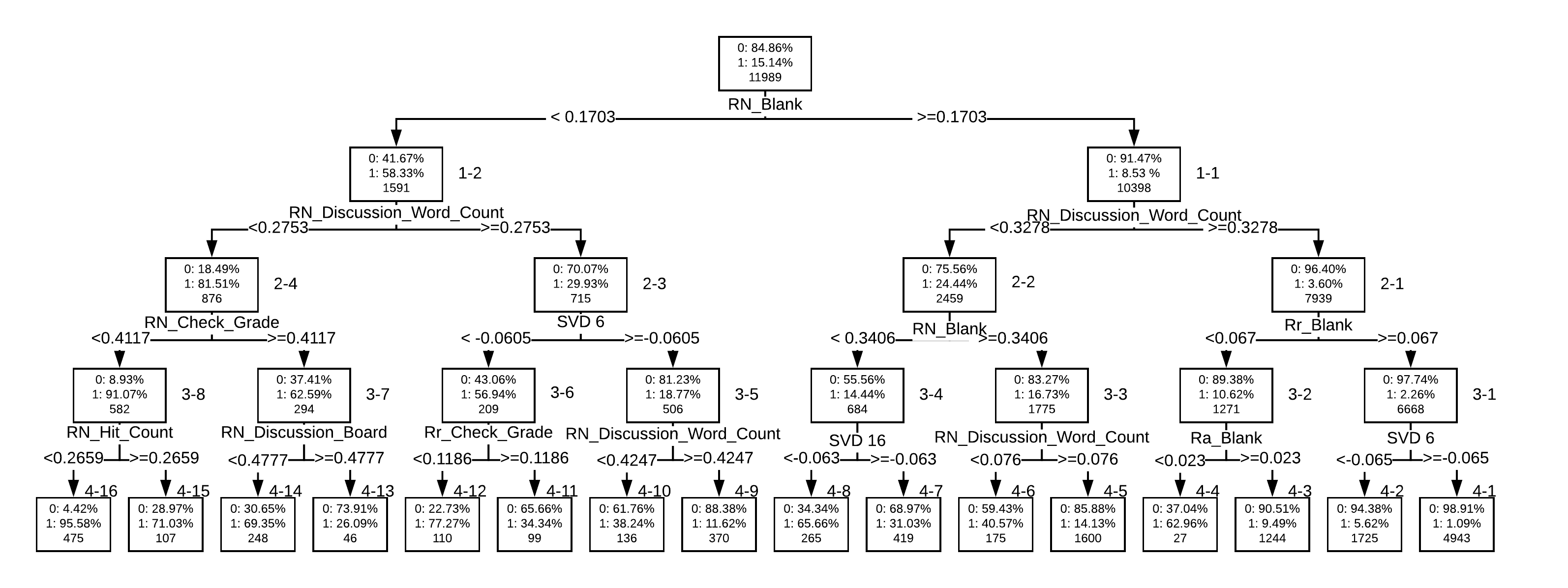
Figure 5. Simulated decision tree model results.Because the decision tree simulates the best model in the round 3 analysis (i.e. behavioral + demographic + discussion contents), some students were removed if they did not have associated discussion content.The decision tree presents the predictive rules with a tree structure. The topmost node shows the original percentages of the students (0: successful students (84.86%); 1: at-risk students (15.14%) and the number of students (11,989). The most important predictor is RN_Blank (Rules 1-1 and 1-2 below), which splits all students into two nodes. RN_Blank represents a student’s ranking on the frequency of the behavior “Blank” which refers to course activities not created with Blackboard’s built-in tools. If RN_Blank’s value is higher or equal to 0.1703, the percentage of successful students grows to 91.47% (the right node, 10,398 students). Oppositely, the percentage of at-risk students grows to 58.33% if the RN_Black’s value is lower than 0.1703. Similarly, RN_discussion_word_counts (Rules 2-3 and 2-4 below), when combined with RN_Blank behaviors (Rule 1-2), is also a predictor for at-risk students. In other words students who accessed materials outside the LMS (ranked lower than 17.03%) and posted fewer words in the discussion forums (ranked lower than 27.53%) had a higher chance of identifying as at-risk.*Rule 1-1: RN_Blank >= 0.1703 (0/1: 0.91/0.09)*Rule 1-2: RN_Blank <0.1703 (0/1: 0.42/0.58)Rule 2-1: 1-1 + RN_discussion_word_counts >=0.3278 (0/1: 0.96/0.04)Rule 2-2: 1-1 + RN_dicussion_word_counts < 0.3278 (0/1: 0.76/0.24)*Rule 2-3: 1-2 + RN_discussion_word_counts >= 0.2753 (0/1: 0.7/0.3)*Rule 2-4: 1-2 + RN_discussion_word_counts <0.2753 (0/1: 0.18/0.82)Rule 3-1: 1-1 + 2-1 + Rr_blank >= 0.067 (0/1: 0.98/0.02)Rule 3-2: 1-1 + 2-1 + Rr_blank < 0.067 (0/1: 0.89/0.11)Rule 3-3: 1-1 + 2-2 + RN_blank >= 0.1703 (0/1: 0.83/0.17)Rule 3-4: 1-1 + 2-2 + RN_blank < 0.1703 (0/1: 0.56/0.44)*Rule 3-5: 1-2 + 2-3 + SVD6 >= -0.0625 (0/1: 0.81/0.19)*Rule 3-6: 1-2 + 2-3 + SVD6 < -0.0625 (0/1: 0.43/0.57)Rule 3-7: 1-2 + 2-4 + RN_check_grade >= 0.4117 (0/1: 0.37/0.63)Rule 3-8: 1-2 + 2-4 + RN_check_grade < 0.4117 (0/1: 0.09/0.91)
Early Warning Signals from Discussion Content
In the text processing, we parsed individual students’ textual discussions into terms then used a dictionary to code student’s textual content terms into a large matrix. The singular-value decomposition (SVD) is a common approach to factorize a complex matrix. We extracted 42 features representing student’s discussion content. This approach has been widely used to extract important content features or group similar content into clusters. The textual feature analysis indicated that SVD 6 was an important feature for identifying at-risk students (Rules 3-5 and 3-6 above). In other words, based on the branches, it appears SVD 6 below a threshold of -0.0605 is an early warning indicator for identifying at-risk students. Therefore, we extracted the textual contents that met this threshold. When looking at the extracted raw textual data, we were able to determine that successful students (those above the threshold > -0.0605) were all enrolled in the Government class while at-risk students (lower than the threshold < -0.0605) were enrolled mostly in the Civics class.Additional variables, including those we derived from domain categorization (discipline, offering, and enrollment), were incorporated into the analysis to further examine why SVD 6 might be an early warning predictor. The results are illustrated in the tables below using a percentage rate of 40% for students meeting the at-risk SVD 6 threshold, along with accuracy and recall rates for each:
First semester courses (see Table 5)
Courses with enrollments less than 20 (see Table 6)
Courses in the History, Geography, and Political Science disciplines (see Table 7)
Specific courses with very high at-risk percentages included Civics, History, and Chemistry (see Table 8). These courses also triangulate with the offering and discipline domain categorization results. Accuracy and recall rates are not available for individual courses.
Table 5.
Offering | At-Risk Threshold (<-0.0605) | Accuracy | Recall |
|---|---|---|---|
AP | 11.25% | 0.920424 | 0.528517 |
O (Other) | 30.92% | 0.904719 | 0.654545 |
S1 (Sem 1) | 42.47% | 0.903352 | 0.715743 |
S2 (Sem 2) | 35.80% | 0.914952 | 0.646840 |
SVD 6 At-Risk Threshold Percentage, Accuracy, and Recall by Course OfferingTable 6.
Enrollment | At-Risk Threshold (<-0.0605) | Accuracy | Recall |
|---|---|---|---|
En1 (0-20) | 52.10% | 0.8992 | 0.5778 |
En2 (21-75) | 29.14% | 0.9090 | 0.6220 |
En3 (76-200) | 31.08% | 0.9257 | 0.7131 |
En4 (>200) | 31.51% | 0.8984 | 0.6461 |
SVD 6 At-Risk Threshold Percentage, Accuracy, and Recall by EnrollmentTable 7.
Discipline | At-Risk Threshold (<-0.0605) | Accuracy | Recall |
|---|---|---|---|
Comp Sci | 34.51% | 0.9071 | 0.5294 |
Earth Sci | 39.94% | 0.8876 | 0.6571 |
Econ | 4.76% | 0.9115 | 0.6159 |
Geography | 76.00% | 0.9600 | 0.6667 |
History | 42.53% | 0.9080 | 0.7040 |
Life sci | 18.93% | 0.9277 | 0.6951 |
Physical sci | 33.14% | 0.8941 | 0.6588 |
Political sci | 64.17% | 0.8969 | 0.5806 |
Social sci | 29.18% | 0.9180 | 0.6416 |
SVD 6 At-Risk Threshold Percentage, Accuracy, and Recall by DisciplineTable 8.
Course | At-Risk Threshold (<-0.0605) | Course | At-Risk Threshold (<-0.0605) | |
|---|---|---|---|---|
American History B | 64.29% | Human Space Exploration | 10.24% | |
Anatomy and Physiology A | 40.05% | Medical Terminology | 5.40% | |
Anatomy and Physiology B | 23.24% | MS Comprehensive Science 1A | 0.00% | |
Anthropology | 37.93% | MS Comprehensive Science 2A | 25.00% | |
AP Art History | 64.71% | MS Comprehensive Science 3A | 11.11% | |
AP Art History | 44.44% | MS World Cultures A | 0.00% | |
AP Biology | 15.57% | Mythology and Folklore: Legendary Tales | 52.08% | |
AP Chemistry | 59.52% | Native American History | 21.37% | |
AP Computer Science A | 22.73% | Oceanography A | 47.38% | |
AP Environmental Science | 3.10% | Oceanography B | 5.26% | |
AP Macroeconomics | 1.21% | Physical Science A | 58.33% | |
AP Microeconomics | 2.08% | Physical Science B | 58.06% | |
AP Physics 1 | 52.29% | Physics A | 51.31% | |
AP Physics C | 25.86% | Physics B | 0.83% | |
AP Psychology | 12.09% | Psychology | 54.81% | |
AP U.S. Government and Politics | 0.00% | Science A | 16.67% | |
AP U.S. History | 5.63% | Science B | 75.68% | |
AP U.S. History B | 3.23% | Sociology A | 5.51% | |
AP World History | 0.89% | Sociology B | 13.66% | |
Archaeology: Detectives of the Past | 31.03% | Sociology I: The Study of Human Relationships | 3.40% | |
Astronomy | 71.85% | Sociology II: Your Social Life | 0.00% | |
Biology A | 69.05% | U.S. History A | 71.60% | |
Biology B | 14.75% | U.S. History and Geography A | 32.50% | |
Chemistry A | 77.21% | U.S. History and Geography B | 39.13% | |
Chemistry B | 84.07% | U.S. History B | 73.68% | |
Civics | 94.99% | Veterinary Science: The Care of Animals | 28.26% | |
Criminology: Inside the Criminal Mind | 14.94% | World Cultures A | 57.14% | |
Earth Science A | 69.57% | World Cultures B | 81.82% | |
Earth Science B | 37.50% | World Geography A | 66.67% | |
Economics | 7.46% | World Geography B | 86.96% | |
Environmental Science A | 58.43% | World History A | 84.75% | |
Environmental Science B | 29.51% | World History and Geography A | 29.55% | |
Forensic Science - Advanced | 1.24% | World History and Geography B | 31.25% | |
Forensic Science - Introduction | 2.02% | World History B | 84.03% | |
Great Minds in Science: Ideas for a New Generation | 45.45% | Human Space Exploration | 10.24% | |
History of the Holocaust | 25.00% | Medical Terminology | 5.40% |
SVD 6 At-Risk Threshold Percentage by Individual CourseNote: Overall average = 31.38%Further investigation into the reasons behind the SVD 6 significance as an at-risk predictor included examining the textual content for clues. One conjecture was that age was a factor in writing ability. Successful students were all enrolled in the Government class while the at-risk students were enrolled mostly in the Civics class, which tends to be a class that is offered earlier in high school and is not as advanced as Government. Also, older students (or even all students) taking the Civics class might already be at-risk and thus demonstrate lower writing ability. (They may be taking the class for credit recovery vs. voluntary enrollment in an advanced Government class.) However, in our analysis students’ ages did not show significant differences between high SVD6 (> -0.0605) and low SVD 6 (< -0.0605) students. It should be noted that the age data included numerous input errors that we were not able to eliminate.Next, we were interested in learning if the content of the text discussions might provide insight into the significance of the SVD 6 feature. We conducted an analysis using results from the LIWC function word analytic tool. The 2015 iteration of LIWC (Pennebaker, Boyd, Jordan, & Blackburn, 2015) (http://liwc.wpengine.com/) contains 90 output variables, including predetermined dimensions, singular function word categories (i.e. pronouns), punctuation, grammatical, mechanical, and other measures to choose from when analyzing text files. Since this was our first foray into the LIWC universe, we limited the results of our text analysis to eight dimensions and measures including word count, analytic, authentic, words per sentence (WPS), six letter words, function words, pronouns, and cognitive process. These dimensions and measures were chosen based on our best guess as to what might help us determine the meaning behind the SVD 6 feature.When we added the LIWC results to our predictive model, our findings indicated that indeed, successful students (in this case all students in the successful group were enrolled in the Government course) used more words that were analytic than those in the at-risk group, which showed the use of more authentic words with greater use of pronouns (indicating more of a focus on themselves versus focus on the content being discussed) (see Table 9). Conjecturing again, the LIWC analysis also showed a much greater word count in the successful group, which along with the analytic focus of that group may be an indication of higher level thinking. Either the course itself requires a higher level of writing skill, or the students within that course may exhibit higher level thinking and writing ability.Table 9.
| Word Count | Analytic | Authentic | WPS | Six Letter Words | Function Words | Pronoun | Cognitive Process |
|---|---|---|---|---|---|---|---|---|
SVD6 at-risk | 149452 | 51.75 | 21.17 | 2197.82 | 18.44 | 55.84 | 14.75 | 15.08 |
SVD6 successful | 216534 | 82.87 | 17.28 | 1691.67 | 25.36 | 50.31 | 10.64 | 13.27 |
LIWC Analysis Results Across Eight DimensionsIdentifying the Best Threshold: Precision and RecallA predictive model usually uses 0.5 as the threshold to determine a case that should be predicted as 1 (the probability of 1 is >=0.5) or as 0 (the probability of 0 is >=0.5; the sum of two probabilities 1 plus 0 is equal to 1). Here we would like to introduce another performance indicator called precision. Precision is the ratio of all predicted positive (i.e. at-risk) cases whose actual values are also positive. Recall is the ratio of positive students being captured by the model. High precision and high recall represent the model that can most precisely predict and capture a high percentage of positive cases. High precision and low recall means the model can precisely predict positive cases, but it can only capture a low percentage of positive cases. Since early warning is the goal of the predictive model, recall rate is more important than precision.In practice, we can increase the recall rate by lowering the threshold. However, when you lower the threshold to increase the number of at-risk students being captured by the model, the action also increases the chance of false positives (FP) (i.e. lower precision rate). Table 10 and Figure 6 show the precision and recall rates at different thresholds. In the dataset from both academic years, there were 2,263 at-risk students and 9,726 successful students. At the threshold 0.5, the recall rate is 0.545. That means 1,233 (2263*0.545) at-risk students can be captured by the model. The precision rate 0.644 means that 1,915 (1233/0.644) students were predicted as at-risk. In other words, 682 (1915-1233) successful students are predicted as at-risk. When we lower the threshold to 0.2, the recall rate increased to 0.648. That means the model can capture up to 1,466 at-risk students. However, at the same time, the precision rate is decreased to 0.529, meaning 865 successful students will be mis-judged as at-risk students. Lowering the threshold can increase the number of at-risk students being captured by the model. However, at the same time, it may increase the burden for support because more successful students will be mis-identified as at-risk. In Figure 6, the cross point represents the most balanced point under the consideration of precision and recall (around 0.31). Therefore, when the model to predict a student’s at-risk probability is implemented, 0.31 should be used for the threshold setting instead of the default 0.5 because it will capture more true positive cases (i.e. at-risk students) and control the increase of false positives. (Details about the implementation of the early warning model can be found in the section on model implementation.) Using this threshold in the model, approximately 59% of at-risk students will be captured, while approximately 59% of predicted students will actually be at-risk. Our goal is to identify as many at-risk students as possible while limiting the number of false positives; and if we use this threshold, the balance is more efficient. If you want to increase the number of at-risk students identified, the threshold may be lowered, but this will increase the number of false positives.Precision or positive predictive value (PPV)PPV = TP__ TP + FPTable 10.
Threshold | Precision | Recall |
|---|---|---|
0.20 | 0.529 | 0.648 |
0.25 | 0.567 | 0.629 |
0.30 | 0.584 | 0.596 |
0.35 | 0.607 | 0.574 |
0.40 | 0.617 | 0.557 |
0.45 | 0.639 | 0.550 |
0.50 | 0.644 | 0.545 |
Precision and Recall Rates at Different Thresholds
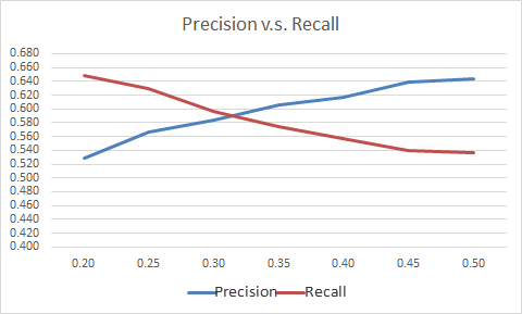
Figure 6. Precision and recall crosspoint.
Discussion
In this project, we explored student behavioral, textual, and limited demographic data retrieved from select courses offered through Michigan Virtual School for the 2014-2015 and 2015-2016 academic years. One overarching goal was determining the type of data we could collect as well as how accurate and comprehensive the data were. We also wanted to explore a variety of data mining analysis techniques, including DL for text analysis and improved prediction accuracy. Finally, we were interested in looking for predictors that could act as early warning indicators for detecting learners that might be at-risk of failure early in the semester.
Data Storage and Collection
Data collection proved to be somewhat challenging at first. Particularly challenging was the ability to perform consistent data retrieval actions/processes so that data from one extraction was matched to data from another extraction by date and type. Data collection processes could be improved by setting up Extract Transform and Load (ETL) to a data warehouse to enable long-term data processing, storage, reporting, and tracking. Davies, et. al (2017) discuss issues with data collection and retrieval at length. One issue is the LMS itself, which is a tool that was designed to host educational materials and content not to measure learners’ interaction with that content. In addition, data systems are typically not integrated in ways that support interoperability across systems, that capture both activity-trace data and process-level data, and that store data for real-time use. Systems should be designed from the beginning with a strategic approach that incorporates data use in the design. In the end, we were able to collect baseline data from a subset of courses over two academic years which included behavioral data from the LMS server logs, final course grades, gender, and text discussion posts linked to student ID. While not an optimal data set, it proved to be enough to test a variety of prediction models and assess their accuracy.
Data Quality
The accuracy and variation in the type of data used are important considerations in EDM. In general, the more varied the data points, the more accurate and reliable the prediction model will be. To increase variability, one approach is to add additional demographic variables such as Socio-Economic Status, GPA, at-risk designation, or course evaluation survey results. Other variations might also include increasing the number of courses in the data set or expanding the collection to include prior years. Variation can serve to improve the predictive power of a model and as a comparison to validate if the accuracy of the prediction remains the same. Data quality is also highly influenced by the accuracy of the data and includes such things as whether or not a variable is representative of a specific behavior. For example, are the activity indicators that register login and log off accurately representative of time spent in the LMS? We provide a more detailed account of data quality, as it relates to this study, below.
Online behavior data
The online behaviors were extracted from the activity accumulator table in Blackboard’s database system. Except for some minor errors (e.g. a small portion of records contained misplaced values), the overall data quality was good. However, there were two major limitations, which decreased the possibility of advanced analysis. First, we were not able to calculate accurate time spent in the course. Blackboard uses a unique session ID to track user logins. However, if a learner did not log off or close the browser right after his/her learning had ended, the session ID would keep the aggregate learner’s time spent on the platform. We did try to calculate time spent for individual sessions but obtained extreme values. In addition, students could download course materials and access them offline. Because time spent between sessions cannot accurately reflect the actual learning time spent in the course, we made the decision to discard time spent variables in the analysis. Second, the internal_handle field in the activity accumulator table stores additional information about the accessed course materials. However, if the materials were not created with Blackboard’s built-in tools, the value of this field shows as “blank.” Therefore, we were able to aggregate the total access frequency but could not further break down course materials by attributes, such as content format.
Student demographics
Student demographics are considered static variables in the analysis as they do not change dynamically the way learning behaviors do. From the aspect of early warning detection and prediction, demographics can serve as early warning signals even before the course starts. However, in this study, neither age nor gender were selected by the predictive model as an important predictor. Although we tested for age, there were some issues with the accuracy of the data. Additional student demographics, such as accumulated GPA (Arnold & Pistilli, 2012), reason to take online courses (Hung, Hsu, & Rice, 2012), ethnicity (Greller & Drachsler, 2012), and parent’s education level (Dubuc, Aubertin-Leheudre, & Karelis, 2017), have been identified as important predictors in the literature and, if included, may also improve the predictive power of the model.
Online discussion content
Student online discussion text was identified as an important predictor in this study. Combining behavioral with textual data as input variables further improved the model’s accuracy. However, in the data collection process, student replies also included content from their original posts, which increased data noise and took significant effort to ameliorate in the data processing. In addition to the discussion contents, interaction records under individual threads were analyzed via social network analysis and by tracking network pattern changes over time. The interactions of individual students were converted into numerical data and used as input variables in the construction of the predictive model.
Deep Learning with Text Data for Improved Prediction Accuracy of At-risk Students
Although EDM is gaining in momentum, DL in educational settings is still relatively new. We were interested in exploring the potential of DL combined with textual data in improving the prediction accuracy of our model. Specifically, we were interested in comparing DL to other ML models as well as exploring the potential of DL combined with textual data in improving prediction accuracy. We found that DL performance was slightly better than other ML models (i.e. SVM with Polynomial kernel) and the inclusion of textual content improved the overall predictive accuracy in identifying at-risk students. Although the percentage was a relatively small increase in prediction power when using DL, this increase adds an additional element of accuracy in our efforts to use data to support learners – in particular, at-risk learners. One limitation was the small data set which prohibited “deeper” levels of analysis using more advanced DL methods. Perhaps the most important finding was our ability to achieve accurate prediction power with a relatively high level of generalizability and stability. The question of generalizability is important because it may allow us to use the model across different contexts. Further testing will be needed to prove this.In addition to an increase in predictive power, we used a surrogate model analysis to assist us in further understanding the DL results. The SVD 6 feature was identified as an important feature for identifying at-risk students. We tried a variety of approaches in examining the raw text from this feature and discovered some commonalities: successful students (those above the threshold > -0.0605) were all enrolled in the Government class, while at-risk students (lower than the threshold < -0.0605) were enrolled mostly in the Civics class. Further analysis of the SVD 6 threshold predictor revealed that first semester courses, courses with 20 or fewer enrollments, and courses in the disciplines of History, Geography and Political Science all demonstrated larger percentages of predicted at-risk students. We even analyzed the raw text data itself to see if we could tease out a meaningful explanation for the importance of this predictor. Although a variety of meanings might be attributed to the underlying cause of this textual feature being identified as a significant predictor in the DL analysis, everything is conjecture at this point. However, its importance may come into play in the support or intervention stage.
Recommendations
Based on our initial data mining explorations with deep learning, we make the following recommendations:
Continue exploring the DL model which resulted in an overall prediction accuracy of 86.9%, a prediction accuracy of 94.5% in identifying successful students, and a 54.5% in identifying at risk students. The results show a slight increase in the accuracy of predicting at-risk students. However, even just 1% additional predictive power is worth the extra effort of DL.
Increase the number of courses used in the data set. The access to course data in the current study was intentionally limited. The model may change with additional course disciplines. It is also the case that if all course data were used, the accuracy might be improved. Smaller data sets prohibit “deeper” levels of analysis using more advanced DL methods.
Seek to advance generalizability of the model. For example, even though it is more challenging, generating relative frequency across courses improves generalizability. However, deriving relative frequency across the limited courses to which we had access required extensive code so deploying across an entire institution would be very complex. There are other ways we can test for generalizability. We could compare results with data from another set of course categories or domains identified as important to the institution, or compare with the entire set of course offerings.
We know SVD 6 is an important association with performance, but we don’t yet know why. Continued research into data mining with the inclusion of text mining would be an important next step. For this study we applied Natural Language Processing (NLP) to the SVD approach to extract the textual features. There are other more advanced methods we can try such as variant auto-coder or t-SNE. New research may also offer further prediction power including the work by Pennebaker, et. al (2014) in using function words as a predictor of success.
Differentiate discussion post text by teacher/student within a single thread if possible to improve the quality of the data (removing noise).
Investigate DL with text mining in real-time Time Series Analysis validation.
When setting parameters for identifying at-risk learners, the limitations of the model suggest that it is better to err on the side of over identifying.
To improve the prediction accuracy and generalizability of the model, identify more variables highly related to the target status. In other words, link data such as demographics which are more typically indicative of at-risk status, such as free and reduced lunch or a school or district level at-risk designation. However, it may be worthwhile to compare models that incorporate this additional data and those that don’t to identify any bias in the algorithm. Labeling or tracking students by profiling can result in the denial of opportunities to underrepresented groups.
The quality of some data was of limited use because of input errors. Providing a drop down with possible choices for student age, rather than allowing students or others to input data by hand is one way to alleviate this problem. Other examples include linking data from one system to another such as additional demographic data with behavioral data in the LMS and linking to other student performance data systems or course evaluation data.
Extracted early warning indicators, including behaviors and number of words posted, suggest that students who accessed materials outside the LMS (ranked lower than 17.03%) and posted fewer words in the discussion forums (ranked lower than 27.53%) had a higher chance of identifying as at-risk.
To improve predictive power in the model, we would suggest collecting more student demographic data at the stage of new student registration.
Although there are some definitive results from this study, educational data mining begins with data selection but results in the development of predictive models that require an iterative revision process to perfect (Davies, et. al, 2017). This initial exploration has added the additional element of textual content to a deep learning approach. The results indicate a positive result for a deep learning approach in educational data mining. With further testing of the model, including expanded course offerings, the inclusion of other data for triangulation, and real-time analytics such as time series analysis, we believe this approach would lead to a highly accurate, generalizable predictive model that would support an early warning system for at-risk learners.
References
Arnold, K. E., & Pistilli, M. D. (2012, April). Course signals at Purdue: Using learning analytics to increase student success. In Proceedings of the 2nd International Conference on Learning Analytics and Knowledge (pp. 267-270). ACM.Bengio, Y. (2012). Deep learning of representations for unsupervised and transfer learning. Journal of Machine Learning Research, 27, 17-37. Retrieved from http://proceedings.mlr.press/v27/bengio12a/bengio12a.pdfDavies, R., Nyland, R., Bodily, R., Chapman, J., Jones, B., & Young, J. (2017). Designing technology-enabled instruction to utilize learning analytics. Techtrends: Linking Research & Practice To Improve Learning, 61(2), 155-161. doi:10.1007/s11528-016-0131-7Du, X., Yang, J., Shelton, B. E., Hung, J. L., & Zhang, M. (2018). Beyond bibliometrics: a systematic meta-review and analysis of learning analytics research. Manuscript submitted to publication.Dubuc, M. M., Aubertin-Leheudre, M., & Karelis, A. D. (2017). Relationship between academic performance with physical, psychosocial, lifestyle, and sociodemographic factors in female undergraduate students. International Journal of Preventive Medicine, 8-22Gašević, D., Dawson, S., Rogers, T., & Gasevic, D. (2016). Learning analytics should not promote one size fits all: The effects of instructional conditions in predicting learning success. The Internet and Higher Education, 28, 68–84. Retrieved from https://www.researchgate.net/publication/312846891_Piecing_the_Learning_Analytics_Puzzle_A_Consolidated_Model_of_a_Field_of_Research_and_PracticeGreller, W., & Drachsler, H. (2012). Translating learning into numbers: A generic framework for learning analytics. Journal of Educational Technology & Society, 15(3), 42-57Hall, P., Phan, W., & Ambati, S. (2017). Ideas on interpreting machine learning. Retrieved from the O’Reilly website: https://www.oreilly.com/ideas/ideas-on-interpreting-machine-learning.Hung, J. L., Hsu, Y. C., & Rice, K. (2012). Integrating data mining in program evaluation of K-12 online education. Journal of Educational Technology & Society, 15(3). 27-41Pennebaker, J.W., Boyd, R.L., Jordan, K., & Blackburn, K. (2015). The development and psychometric properties of LIWC2015. Austin, TX: University of Texas at Austin.Pennebaker, J. W., Chung, C. K., Frazee, J., Lavergne, G. M., & Beaver, D. I. (2014). When Small Words Foretell Academic Success: The Case of College Admissions Essays. PLoS ONE, 9(12), 1-10. doi:10.1371/journal.pone.0115844Powers, D. M. (2011). Evaluation: from precision, recall and F-measure to ROC, informedness, markedness and correlation, Journal of Machine Learning Technologies, 2(1), 37–63.Raczko, E., & Zagajewski, B. (2017) Comparison of support vector machine, random forest and neural network classifiers for tree species classification on airborne hyperspectral APEX images. European Journal of Remote Sensing, 50(1), 144-154.Schmidhuber, J. (2015). Deep learning in neural networks: An overview. Neural Networks, 61 85–117. https://arxiv.org/pdf/1404.7828.pdfSmolyakov, V. (2017). Ensemble learning to improve machine learning results [Blog post]. Stats and Bots. Retrieved from https://blog.statsbot.co/ensemble-learning-d1dcd548e936Tausczik, Y. R., & Pennebaker, J. W. (2010). The psychological meaning of words: LIWC and computerized text analysis methods. Journal of Language and Social Psychology, 29(1), 24-54. Retrieved from https://www.cs.cmu.edu/~ylataus/files/TausczikPennebaker2010.pdf
Appendix A
2014-2015 | Discipline | Offering | Enrollments |
| 2015-2016 | Discipline | Offering | Enroll-ments |
|---|---|---|---|---|---|---|---|---|
American History 1A | history | S1 | En2 | American History A | history | S1 | En2 | |
American History A | history | S1 | En1 | American History B | history | S2 | En2 | |
American History B | history | S2 | En2 | Anatomy and Physiology A | life sci | S1 | En4 | |
Anatomy and Physiology A | life sci | S1 | En4 | Anatomy and Physiology B | life sci | S2 | En3 | |
Anatomy and Physiology B | life sci | S2 | En3 | Anthropology | social sci | O | En3 | |
AP Art History | history | AD | En1 | AP Art History | history | AD | En2 | |
AP Art History v10 | history | S1 | En2 | AP Biology | life sci | AD | En3 | |
AP Biology | life sci | AD | En2 | AP Chemistry | physical sci | AD | En2 | |
AP Biology Sem 1 | life sci | S1 | En2 | AP Chemistry Sem 1 | physical sci | AD | En1 | |
AP Chemistry Sem 1 | physical sci | S1 | En1 | AP Computer Science A | physical sci | AD | En4 | |
AP Chemistry-dry labs | physical sci | AD | En1 | AP Environmental Science | earth sci | AD | En3 | |
AP Computer Science A | comp Sci | S1 | En2 | AP Macroeconomics | econ | AD | En3 | |
AP Computer Science A Sem 1 | comp Sci | AD | En3 | AP Microeconomics | econ | AD | En3 | |
AP Environmental Science | earth Sci | AD | En2 | AP Physics 1 | physical sci | AD | En2 | |
AP MacroEcon | econ | AD | En2 | AP Physics 1A | physical sci | AD | En2 | |
AP Macroeconomics | econ | AD | En2 | AP Physics C | physical sci | AD | En3 | |
AP MicroEcon | econ | AD | En2 | AP Psychology | social sci | AD | En3 | |
AP Microeconomics | econ | AD | En2 | AP U.S. Government and Politics | political sci | AD | En3 | |
AP Physics 1 Sem 1 | physical sci | S1 | En3 | AP U.S. History | history | AD | En3 | |
AP Physics 1B | physical sci | AD | En2 | AP World History | history | AD | En2 | |
AP Physics C | physical sci | AD | En2 | Archaeology: Detectives of the Past | earth sci | O | En2 | |
AP Physics C Mechanics Sem 1 | physical sci | S1 | En2 | Astronomy | physical sci | O | En4 | |
AP U.S. Government and Politics | political sci | AD | En2 | Biology A | life sci | S1 | En2 | |
AP US Govt and Politics | political sci | AD | En2 | Biology B | life sci | S2 | En2 | |
AP US History | history | AD | En2 | Chemistry A | physical sci | S1 | En2 | |
AP US History B | history | S2 | En2 | Chemistry B | physical sci | S2 | En2 | |
AP World History | history | AD | En2 | Civics | political sci | O | En4 | |
AP World History Sem 1 | history | AD | En2 | Civics Sem-Tri | political sci | O | En1 | |
Astronomy | physical sci | O | En4 | Criminology: Inside the Criminal Mind | social sci | O | En4 | |
Biology A | life sci | S1 | En3 | Earth Science A | earth sci | S1 | En2 | |
Biology B | life sci | S2 | En2 | Earth Science B | earth sci | S2 | En1 | |
Chemistry A | physical sci | S1 | En3 | Economics | econ | O | En4 | |
Chemistry B | physical sci | S2 | En3 | Environmental Science A | earth sci | S1 | En3 | |
Civics | political sci | O | En4 | Environmental Science B | earth sci | S2 | En2 | |
Earth Science A | earth Sci | S1 | En2 | Forensic Science | physical sci | O | En4 | |
Earth Science B | earth Sci | S2 | En2 | Great Minds in Science: Ideas for a New Generation | comp sci | O | En1 | |
Economics | econ | O | En4 | History of the Holocaust | history | O | En2 | |
Environmental Science A | earth Sci | S1 | En3 | Human Space Exploration | physical sci | O | En3 | |
Environmental Science B | earth Sci | S2 | En2 | Medical Terminology | life sci | O | En4 | |
Forensic Science | physical sci | O | En4 | Mythology and Folklore: Legendary Tales | social sci | O | En3 | |
Forensic Science - Advanced | physical sci | AD | En1 | Native American History | political sci | O | En2 | |
Forensic Science - Introduction | physical sci | O | En4 | Oceanography A | earth sci | S1 | En4 | |
Human Space Exploration | physical sci | O | En2 | Oceanography B | earth sci | S2 | En2 | |
Medical Terminology | life sci | O | En4 | Physical Science A | physical sci | S1 | En2 | |
Medical Terminology - | life sci | O | En2 | Physical Science B | physical sci | S2 | En2 | |
MS Comprehensive Science 1A | comp sci | S1 | En1 | Physics A | physical sci | S1 | En3 | |
MS Comprehensive Science 2A | comp sci | S1 | En1 | Physics B | physical sci | S2 | En3 | |
MS Comprehensive Science 2B | comp sci | En1 | Psychology | social sci | O | En4 | ||
MS Comprehensive Science 3A | comp sci | S1 | En1 | Science A | comp sci | S1 | En2 | |
MS World Cultures A | political sci | S1 | En1 | Science B | comp sci | S2 | En2 | |
Native American History | political sci | O | En2 | Sociology A | social sci | S1 | En4 | |
Oceanography A | earth Sci | S1 | En4 | Sociology B | social sci | S2 | En3 | |
Oceanography B | earth Sci | S2 | En2 | U.S. History and Geography A | history | S1 | En3 | |
Physical Science A | physical sci | S1 | En2 | U.S. History and Geography B | history | S2 | En3 | |
Physical Science B | physical sci | S2 | En1 | U.S. History B | history | S2 | En1 | |
Physics A | physical sci | S1 | En3 | US History | history | O | En1 | |
Physics B | physical sci | S2 | En1 | US History B | history | S2 | En1 | |
PhysicsB | physical sci | S2 | En2 | Veterinary Science: The Care of Animals | life sci | O | En3 | |
Psychology | social sci | O | En4 | World Cultures A | political sci | S1 | En1 | |
Science A | comp Sci | S1 | En1 | World Cultures B | political sci | S2 | En1 | |
Science B | comp Sci | S2 | En2 | World Geography A | geography | S1 | En1 | |
Sociology A | social sci | S1 | En3 | World Geography B | geography | S2 | En1 | |
Sociology B | social sci | S2 | En3 | World History A | history | S1 | En1 | |
Sociology I: The Study of Human Relationships | social sci | S1 | En3 | World History and Geography A | history | S1 | En3 | |
Sociology II: Your Social Life | social sci | S2 | En1 | World History and Geography B | history | S2 | En3 | |
U.S. History A | history | S1 | En2 | World History B | history | S2 | En2 | |
U.S. History B | history | S2 | En1 |
| ||||
United States History A v12 | history | S1 | En2 |
| ||||
United States History B | history | S2 | En2 |
| ||||
United States History B v12 | history | S2 | En1 |
| ||||
World Cultures B | political sci | S2 | En1 |
| ||||
World Geography A | geography | S1 | En1 |
| ||||
World Geography B | geography | S2 | En1 |
| ||||
World History A | history | S1 | En3 |
| ||||
World History B | history | S2 | En3 |
|
Consolidated Domain Categories